Aboveground Net Primary Productivity (ANPP) and rainfall in two ecological sites of the Dry Puna (Cobres-Salta, Argentina)

---

First, I load the libraries:

library(tidyverse)
library(readxl)
library(patchwork)
library(ggview)
library(ggrepel)
library(gtsummary)
library(gt)
library(ggpmisc) # Para agregar la ecuación de la recta a cada faceta
library(broom)
library(sessioninfo)

And then I load the dataset, clean it, and make a few edits:

cobres_nueva <- read_excel("ANPP_Precipitaciones Oct Marz.xlsx", sheet = "Cobres_R") # esta es la nueva, con precipitaciones extrapoladas


cobres_nueva <- cobres_nueva %>% 
  mutate(
    sitio2 = factor(sitio, labels = c("Shrub\nsteppe", "Grass-shrub\nsteppe"))
         )

1 Rainfall

The following analyses use rainfall estimated by Gaitán and Biancari (2024), method 2. On average, for each growing season (October to March), rainfall was 150.27 mm, with relatively low variability (CV = 18%), compared to the variability in ANPP.

cobres_nueva %>% 
  filter(sitio == "Campo") %>%
  summarise(
    media = round(mean(precip_gaitan_2, na.rm = T),2),
    sd = round(sd(precip_gaitan_2, na.rm = T),2),
    CV = round(sd/media*100,2),
    min = round(min(precip_gaitan_2, na.rm = T),2),
    max = round(max(precip_gaitan_2, na.rm = T),2)
  ) %>% 
  gt()

Table 1: Summary statistics of growing season rainfall in the harvest year (extrapolated with GEE).

media	sd	CV	min	max
150.27	26.98	17.95	117.66	207.49

2 ANPP in both ecological sites

Because this report targets a broad audience that may not be familiar with the Puna and its environments, it’s convenient to refer to the ecological sites in more general, structural terms. Cerro corresponds to a grass–shrub steppe on steep slopes, and Campo to a shrub steppe on flats. I used these shorter labels in the figures.

2.1 Descriptive analysis

I summarize ANPP for both steppe types with a boxplot, also showing the arithmetic mean and the ANPP values for each year (gray points).

# Calculamos las medias de PPAN por sitio
# medias_ppna <- cobres_nueva %>%
#   group_by(sitio) %>%
#   summarise(media = mean(ppna, na.rm = TRUE))

# Graficamos
ggplot(cobres_nueva, aes(x = sitio2, y = ppna, fill = sitio)) +
  geom_boxplot(
    width = 0.4, outliers = F,
    show.legend = F) +
  geom_point(
    size = 2,
    width = 0.1, 
    height = 0,
    alpha = 0.5,
    position = position_jitter(width = 0.06, seed = 123),
    show.legend = F) +
  stat_summary(
    geom = "point",
    fun = "mean", 
    shape = 23,
    size = 3,
    fill = "white") +
  # Colocamos el texto con geom_text_repel y curvamos la línea de conexión
  # geom_text_repel(
  #   data = medias_ppna,
  #   aes(x = sitio, y = media, label = round(media, 1)),
  #   size = 2.5, color = "black", box.padding = 0.5, max.overlaps = 10,
  #   nudge_x = 0.5, nudge_y = 100,
  #   segment.linetype = "dashed"
  # ) +
  labs(
    y = expression(paste("ANPP (kg MS·", ha^{-1}, "·", año^{-1})),
    x = ""
  ) +
  scale_fill_manual(values = c("#fdae6b", "#a1d99b")) +
  scale_y_continuous(
    limits = c(0, 2000),
    breaks = seq(0, 2000, 500)
  ) +
  theme_bw()

# ggview(width = 3, height = 3)
ggsave("Fig_cajas_medias.png", width = 3.5, height = 3.5, dpi = 600)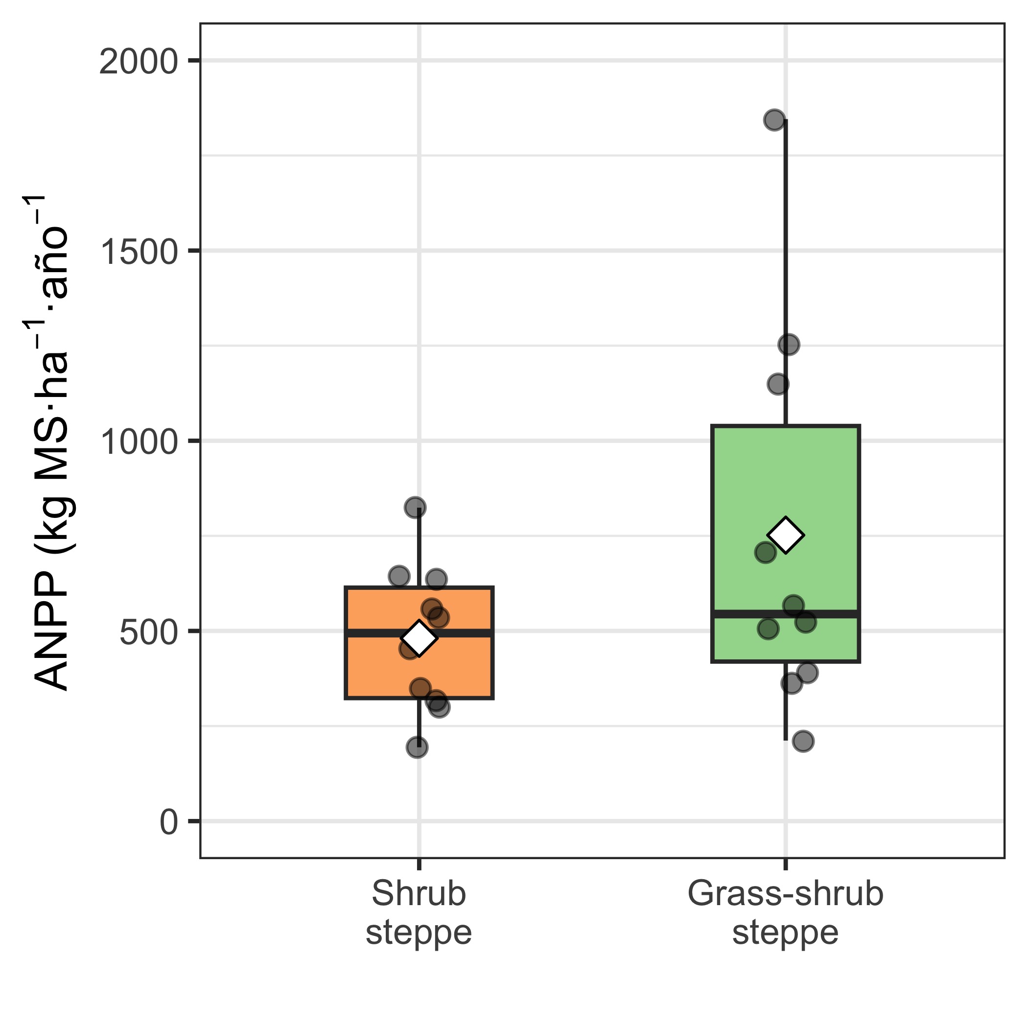

Figure 1: ANPP in both steppes. Points show annual estimates; the horizontal line within each box indicates the median, and the white diamond the arithmetic mean.

Heads up…

What we see in the sample cannot necessarily be generalized to the population. For that, we need Statistical Inference.

2.2 Inferential analysis

The average ANPP in the grass–shrub steppe (751.8 kg DM/ha/year) was 1.6 times higher than in the shrub steppe (480.7 kg DM/ha/year), and this difference was marginally significant (Table 2). ANPP variability in the grass–shrub steppe (CV = 67.7%; Range: 211.7–1845.7 kg DM/ha/year) was higher than in the shrub steppe (CV = 40.3%; Range: 194.1–824.1 kg DM/ha/year)(Figure 1)(Bartlett’s K-squared = 6.96, df = 1, p = 0.008).

# Realiza el análisis y extrae solo el valor t y el valor p
resultado_ttest <- cobres_nueva %>%
  select(fecha2, sitio, ppna) %>%
  pivot_wider(names_from = sitio, values_from = ppna, names_prefix = "ppna_") %>%
  summarize(t_test = list(t.test(ppna_Campo, ppna_Cerro, paired = TRUE, alternative = "less"))) %>%
  pull(t_test) %>%
  purrr::map_df(~tibble(
    estadistico_t = .x$statistic,
    p_value = .x$p.value
  ))

# Crea la tabla elegante con gt

resultado_ttest %>%
  gt() %>%
  tab_header(
    title = "Paired t-test"
  ) %>%
  cols_label(
    estadistico_t = "t",
    p_value = "p-value"
  ) %>%
  fmt_number(
    columns = vars(estadistico_t, p_value),
    decimals = 3
  )

Table 2: Mean ANPP comparison between the two steppes.

Paired t-test
t	p-value
−1.698	0.062

Summing up ANPP…

The grass–shrub steppe tended to be more productive (difference marginally significant) and more variable than the shrub steppe.

3 ANPP across years, by ecological site, and rainfall

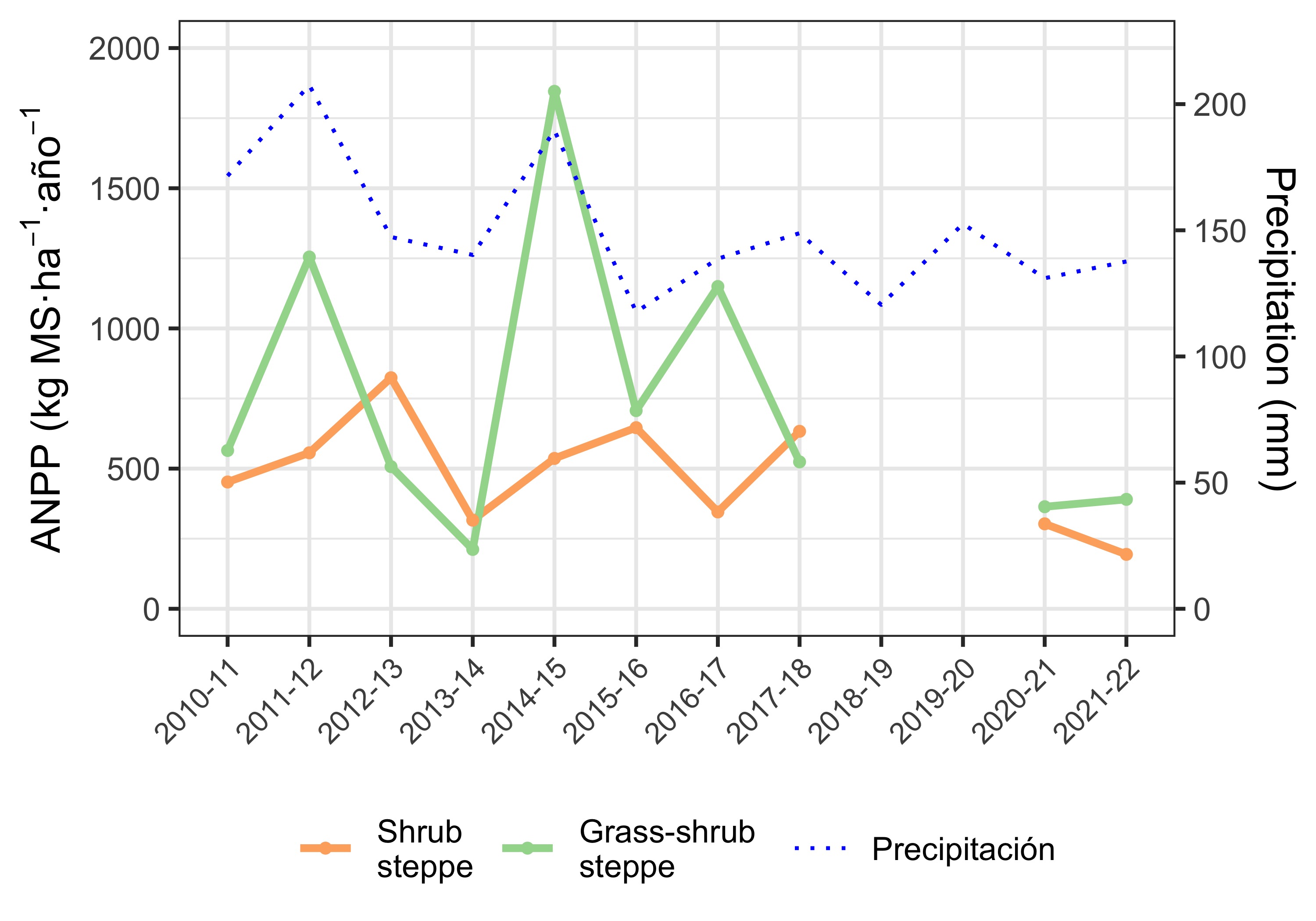
Between the two visualizations (Figure 2 and Figure 3), Figure 3 is more informative, since it doesn’t make sense to facet Campo and Cerro into separate panels.

cobres_nueva %>%
    ggplot(aes(x = fecha2)) +
    facet_wrap(~sitio2) +
    geom_col(aes(y = ppna, fill = sitio), show.legend = FALSE) +
    geom_line(aes(y = precip_gaitan_2 * 9,
                group = sitio,
                color = "Precipitación"),
            size = 0.5) +  
    scale_y_continuous(
      name = expression(paste("ANPP (kg MS·", ha^{-1}, "·", año^{-1})),
      limits = c(0, 2000),  
      sec.axis = sec_axis(~ . / 9, name = "Precipitation (mm)")) +
      theme_bw() +
    theme(axis.text.x = element_text(angle = 45, hjust = 1, size = 8)) +
    labs(
      # title = "Con precipitaciones en la estación de crecimiento (GEE)",
      x = NULL,
      y = expression(PPAN~"(Kg MS / año)")
    ) +
    scale_fill_manual(values = c("#fdae6b", "#a1d99b")) +
    scale_color_manual(values = "blue") +
    theme(
      axis.title.y.left = element_text(color = "black"),
      axis.title.y.right = element_text(color = "black"),
      legend.position = "bottom"
    )

Figure 2: Net Aboveground Primary Productivity (ANPP) in both steppes from 2010 to 2022, with growing season rainfall extrapolated from Gaitán and Biancari (2024).

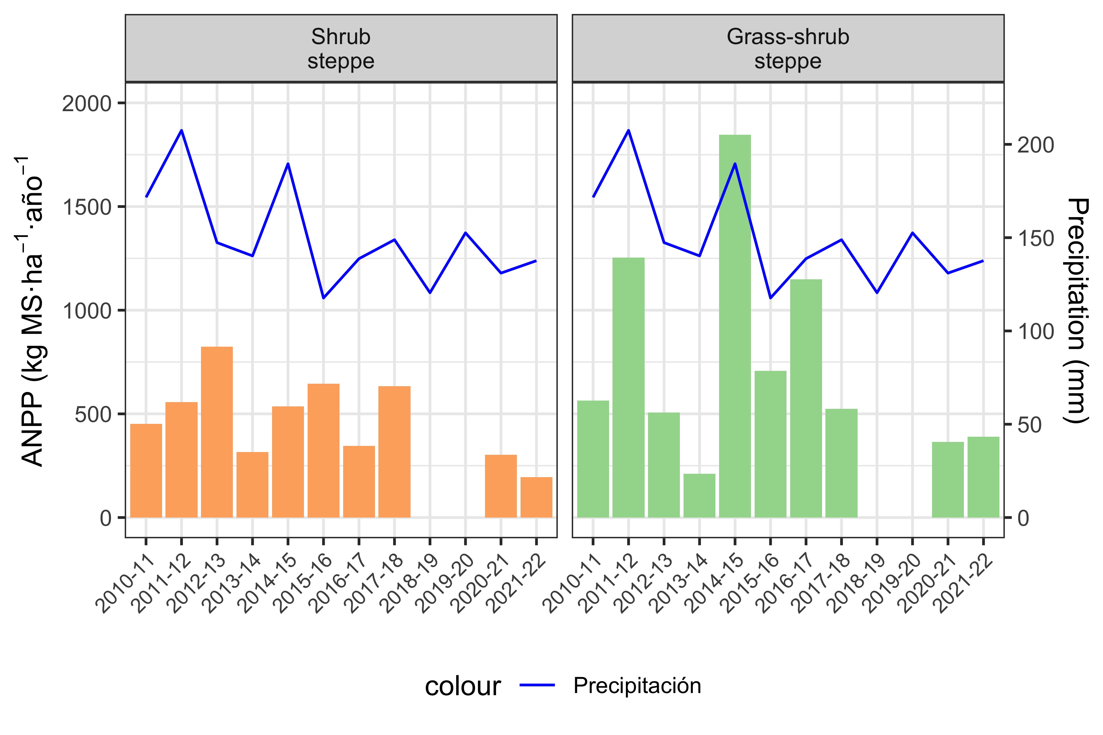
As Mariana mentioned in the WhatsApp group, ANPP’s response to rainfall differs by ecological site in the analyzed sample. In the grass–shrub steppe, ANPP closely follows rainfall in that growing season. In contrast, the shrub steppe’s response is delayed by one year: it depends on rainfall from the previous growing season (Figure 3).

cobres_nueva %>%
  ggplot(aes(x = fecha2)) +
  geom_line(aes(y = ppna, color = sitio2, group = sitio2),
            size = 1,
            na.rm = TRUE) +  # PPAN como línea
  geom_point(aes(y = ppna, color = sitio2, group = sitio2),
             size = 1,
             na.rm = TRUE) +  # PPAN como línea
  geom_line(
    aes(
      y = precip_gaitan_2 * 9,
      group = sitio,
      color = "Precipitación"
    ),
    size = 0.5,
    linetype = "dotted"
  ) +  # Precipitaciones como línea
  scale_y_continuous(
    # name = expression(PPAN ~ "(Kg MS / año)"),
    limits = c(0, 2000),
    sec.axis = sec_axis(~ . / 9, name = "Precipitation (mm)")) +
  theme_bw() +
  theme(axis.text.x = element_text(
    angle = 45,
    hjust = 1,
    size = 8
  )) +
  labs(x = NULL,
       y = expression(paste("ANPP (kg MS·", ha^{-1}, "·", año^{-1})),
       color = NULL,
       # subtitle = "Precipitación de la estación de crecimiento (GEE)"
       ) +
  scale_color_manual(values = c("#fdae6b", "#a1d99b", "blue")) +  # Mismos colores que antes, agregando "blue" para Precipitación
  theme(
    axis.title.y.left = element_text(color = "black"),
    axis.title.y.right = element_text(color = "black"),
    legend.position = "bottom"
  )

Figure 3: Net Aboveground Primary Productivity (ANPP) in both steppes from 2010 to 2022, with growing season rainfall extrapolated from Gaitán and Biancari (2024).

Eduardo suggested adding standard error bars on top of each bar (which represents the mean of the 3 exclosures). It’s a good suggestion; the updated plot can be seen in Figure 4.

cobres_nueva %>%
  ggplot(aes(x = fecha2, y = ppna, fill = sitio2, group = sitio2)) +
  geom_col(position = position_dodge(0.9), na.rm = TRUE) +  # Barras de PPNA
  geom_errorbar(aes(ymin = ppna, ymax = ppna + ppna_se),
                width = 0.1, 
                position = position_dodge(0.9), na.rm = TRUE, color = "grey50") +  # Barras de error alineadas
  geom_line(
    aes(
      y = precip_gaitan_2 * 9,
      group = sitio2,
      color = "Precipitación"
    ),
    size = 0.5,
    linetype = "dotted"
  ) +  # Precipitaciones como línea
  scale_y_continuous(
    # name = expression(PPAN ~ "(Kg MS / año)"),
    limits = c(0, 2500),
    sec.axis = sec_axis(~ . / 9, name = "Precipitation (mm)")
  ) +
  theme_bw() +
  theme(axis.text.x = element_text(
    angle = 45,
    hjust = 1,
    size = 8
  )) +
  labs(x = NULL,
       y = expression(paste("ANPP (kg MS·", ha^{-1}, "·", año^{-1})),
       fill = NULL, color = NULL,
       # subtitle = "Precipitación de la estación de crecimiento (GEE)"
       ) +
  scale_fill_manual(values = c("#fdae6b", "#a1d99b")) +  
  scale_color_manual(values = "blue") +  
  theme(
    axis.title.y.left = element_text(color = "black"),
    axis.title.y.right = element_text(color = "black"),
    legend.position = "bottom"
  )

ggsave("Fig_barras_con_errores.png", width = 5, height = 3.5, dpi = 600)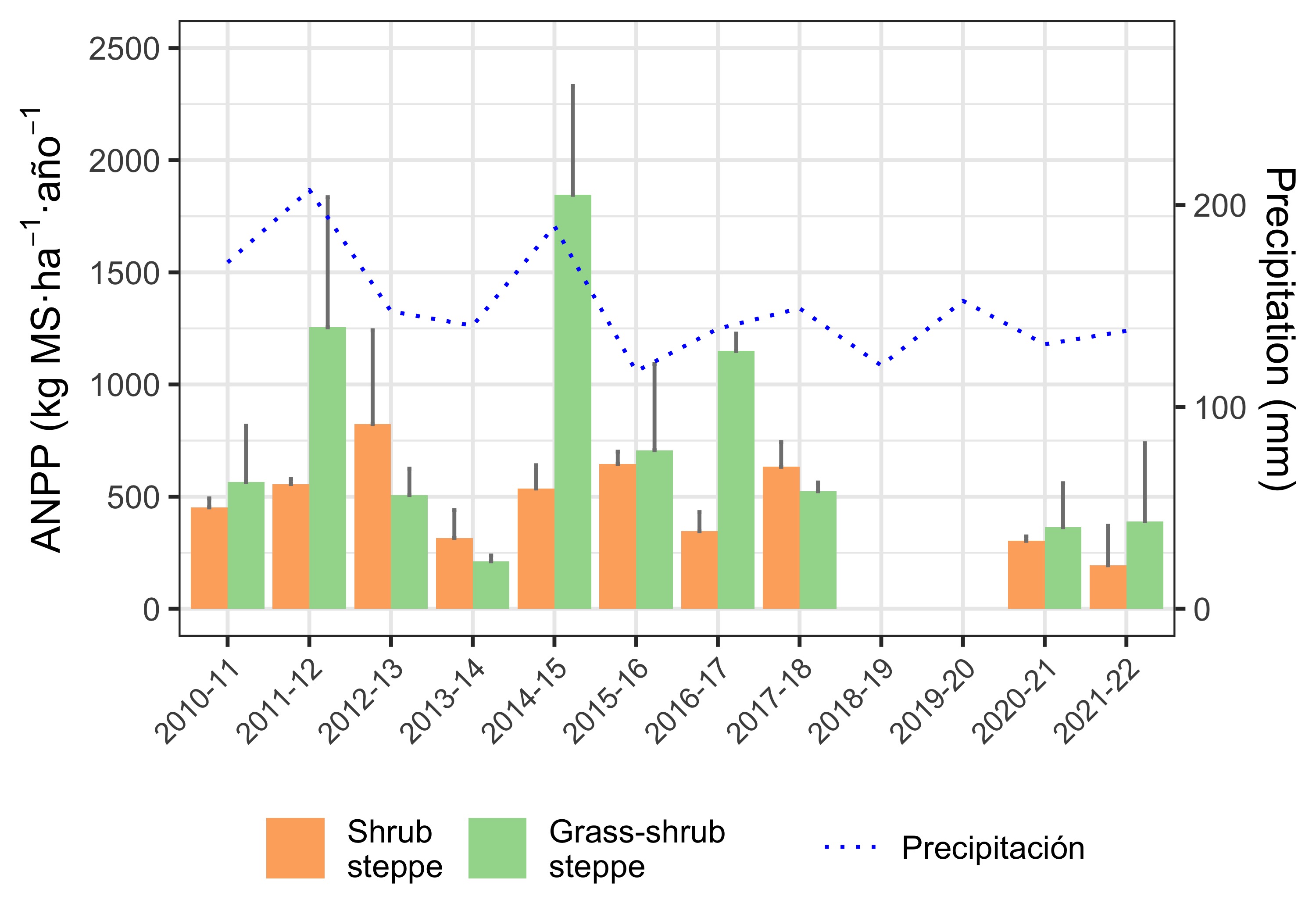

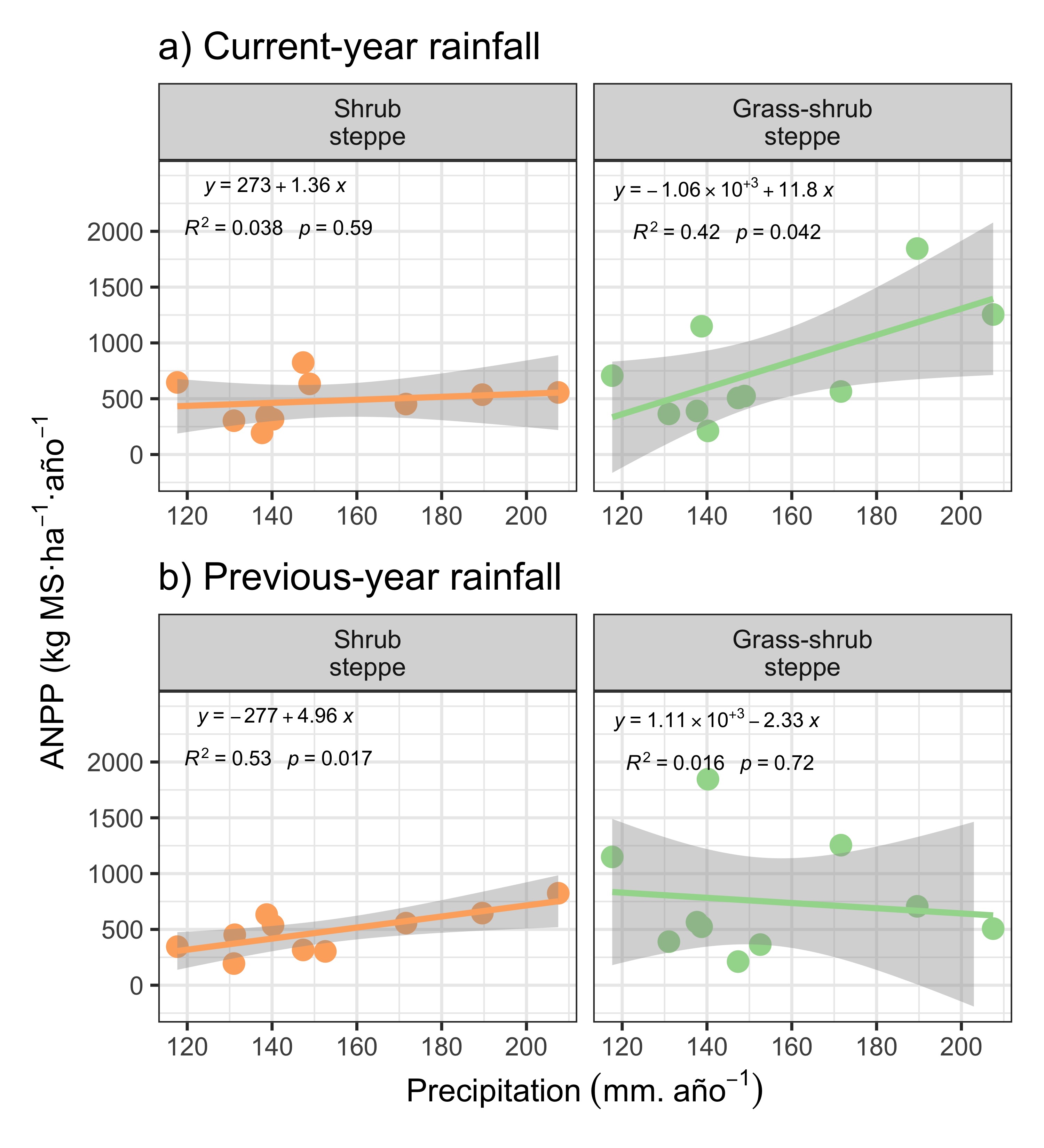
Figure 4: Net Aboveground Primary Productivity (ANPP) in both steppes from 2010 to 2022, with growing season rainfall extrapolated from Gaitán and Biancari (2024).

4 Relationship between ANPP and rainfall

4.1 Descriptive analysis

When analyzing the relationship between ANPP and rainfall during the harvest-year growing season, we find—as mentioned above—no relationship in the shrub steppe. In contrast, for the grass–shrub steppe there is a clear positive relationship in the analyzed sample. This indicates that ANPP depends linearly on rainfall during the same growing season in which ANPP was estimated (Figure 5).

cobres_nueva %>%
   ggplot(aes(
     x = precip_gaitan_2,
     y = ppna)
   ) +
   facet_wrap(~sitio2, 
              # scales = "free_y"
              ) +
   geom_point(aes(color = sitio2),
              size = 3,
              show.legend = F) +
   scale_y_continuous(
     # limits = c(0, 2000)
   ) +
   geom_smooth(aes(color = sitio2),
               method = "lm",
               # se = F, 
               show.legend = F) +
   theme_bw() +
   labs(
     x = "Growing season rainfall in the harvest year",
     y = expression(paste("ANPP (kg MS·", ha^{-1}, "·", año^{-1}))
   ) +
   scale_color_manual(values = c("#fdae6b", "#a1d99b"))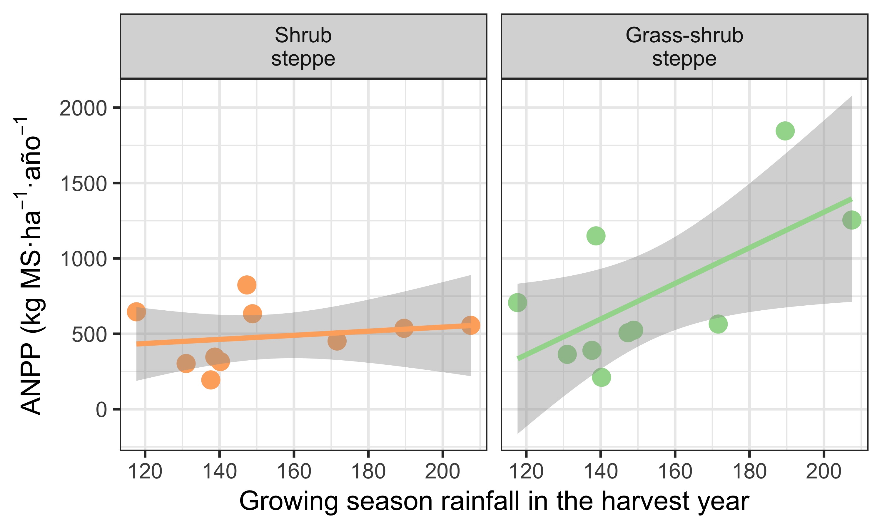

Figure 5: Relationship between Net Aboveground Primary Productivity (ANPP) in both steppes and growing season rainfall extrapolated from Gaitán and Biancari (2024).

Exploring the relationship with rainfall from the previous growing season, the pattern reverses. In the shrub steppe, the relationship becomes positive: there is higher ANPP when it rained more in the previous growing season. In contrast, for the grass–shrub steppe there is no clear relationship (Figure 6).

cobres_nueva %>%
   ggplot(aes(
     x = precip_estacion_anterior_g2,
     y = ppna)
   ) +
   facet_wrap(~sitio2, 
              # scales = "free_y"
              ) +
   geom_point(aes(color = sitio2),
              size = 3,
              show.legend = F) +
   scale_y_continuous(
     # limits = c(0, 2000)
   ) +
   geom_smooth(aes(color = sitio2),
               method = "lm",
               # se = F, 
               show.legend = F) +
   theme_bw() +
  labs(
    x = "Growing season rainfall in the previous year",
    y = expression(paste("ANPP (kg MS·", ha^{-1}, "·", año^{-1}))
  ) +
  scale_color_manual(values = c("#fdae6b", "#a1d99b"))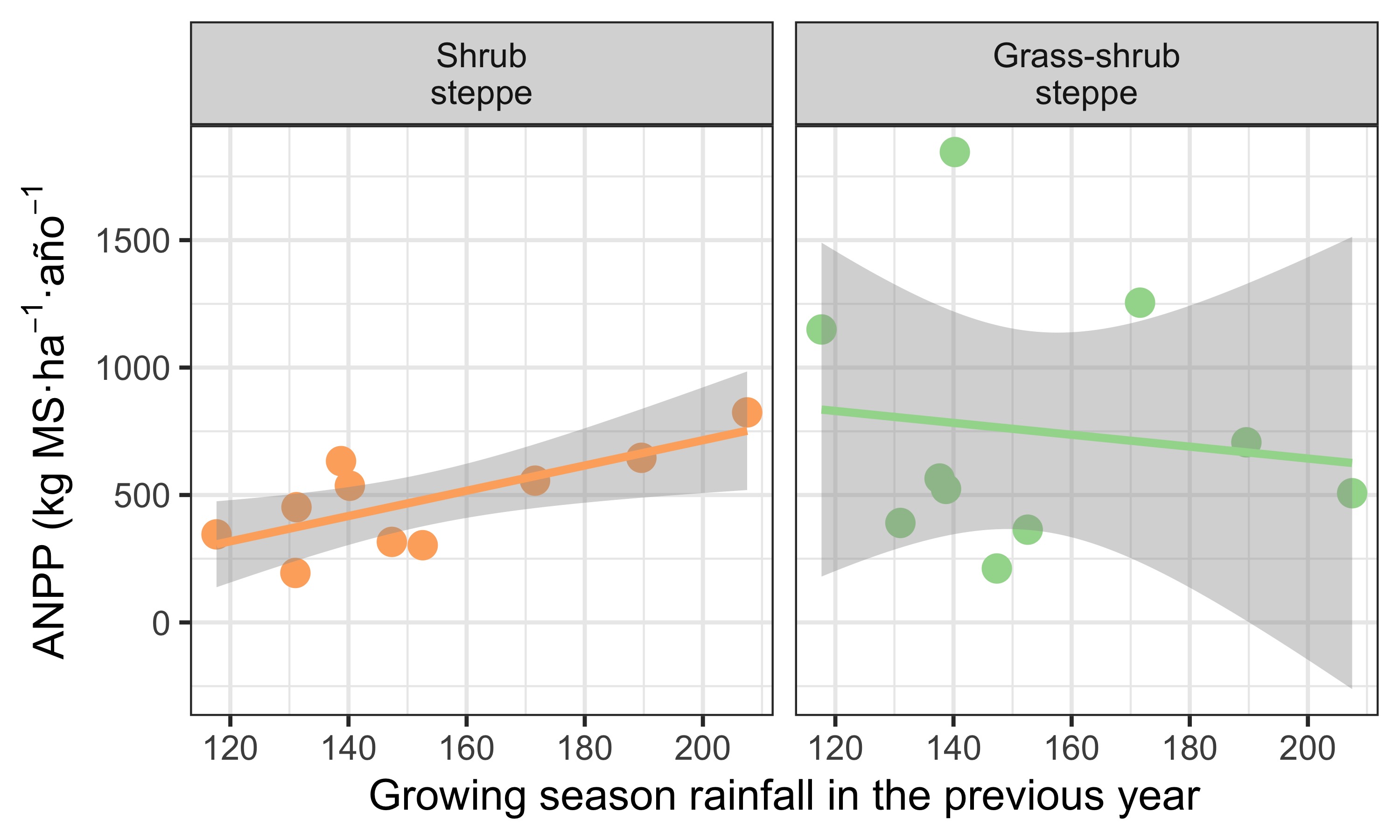

Figure 6: Relationship between Net Aboveground Primary Productivity (ANPP) in both steppes and growing season rainfall from the previous year, extrapolated from Gaitán and Biancari (2024).

Interesting…

ANPP in the grass–shrub steppe responds to what it rained that same year, whereas ANPP in the shrub steppe responds to what it rained the previous year.

Up to this point, we’ve looked at relationships in this sample of exclosures and years. To determine whether these trends can be extrapolated to the population, we use statistical inference. That means testing whether the relationship is statistically significant; note that “significant” does not always mean “important.”

Heads up…

What we see in the sample cannot necessarily be generalized.

When testing the model for ANPP with rainfall during the harvest-year growing season, we see no significant linear regression in the shrub steppe (b = 1.4, P = 0.6) (Table 3). In contrast, in the grass–shrub steppe there is a statistically significant regression, meaning we can extrapolate to the population of sites in the grass–shrub steppe (b = 12; P = 0.042).

The slope—representing the effect of harvest-year growing season rainfall on ANPP—is positive. This means that for each mm of rain in the grass–shrub steppe, ANPP increases by 12 kg DM/ha/year (Table 3). This value is the point estimate of rainfall’s effect on ANPP, and the 95% confidence interval indicates the effect could be between 0.54 and 23 kg DM/ha/year. The model fit is moderate, with \(R^2\) = 42.2%.

# Ajustar modelos
model_campo <- lm(ppna ~ precip_gaitan_2, data = subset(cobres_nueva, sitio == "Campo"))
model_cerro <- lm(ppna ~ precip_gaitan_2, data = subset(cobres_nueva, sitio == "Cerro"))

# summary(model_campo)
# summary(model_cerro)

# Crear tablas de resumen con R² en notas al pie
tabla_campo <- tbl_regression(model_campo, label = list(precip_gaitan_2 ~ "Current-year rainfall")) %>%
  modify_header(label ~ "**Predictor**")

tabla_cerro <- tbl_regression(model_cerro, label = list(precip_gaitan_2 ~ "Current-year rainfall")) %>%
  modify_header(label ~ "**Predictor**")

# Combinar tablas
tabla_merged <- tbl_merge(
  tbls = list(tabla_campo, tabla_cerro),
  tab_spanner = c("Shrub steppe", "Grass-shrub steppe")
)

# Agregar R² como fila adicional

# Convertir tabla a objeto gt, si no lo es ya
tabla_gt <- as_gt(tabla_merged)


# Agregar el R² en el encabezado
tabla_gt %>%
  tab_header(
    title = "Linear models results",
    subtitle = sprintf("R² shrub = %.3f | R² grass-shrub = %.3f", 
                       summary(model_campo)$r.squared, 
                       summary(model_cerro)$r.squared)
  )

Table 3: Linear regression between Net Aboveground Primary Productivity (ANPP) in both steppes and growing season rainfall in the harvest year, extrapolated from Gaitán and Biancari (2024). Beta represents the estimated effect (regression slope).

Linear models results
R² shrub = 0.038 | R² grass-shrub = 0.422
Predictor	Shrub steppe			Grass-shrub steppe
	Beta	95% CI	p-value	Beta	95% CI	p-value
Current-year rainfall	1.4	-4.2, 6.9	0.6	12	0.54, 23	0.042
Abbreviation: CI = Confidence Interval

When I fit the ANPP model with rainfall from the previous growing season, the results flip. For the shrub steppe, there is a significant regression (b = 5.0; P = 0.017) (Table 4), whereas for the grass–shrub steppe we cannot claim a significant regression (b = -2.3; P = 0.7).

In the shrub steppe, the effect of previous growing season rainfall on ANPP is positive. The slope interpretation is that for each mm of rain in the shrub steppe, ANPP increases by 5 kg DM/ha/year (Table 4). This is the point estimate of rainfall’s effect on ANPP in the shrub steppe, and the 95% confidence interval indicates the effect may be between 1.1 and 8.8 kg DM/ha/year. Similarly, the model fit is moderate, with \(R^2\) = 52.9%.

# Ajustar modelos de regresión
model_campo <- lm(ppna ~ precip_estacion_anterior_g2, data = subset(cobres_nueva, sitio == "Campo"))
model_cerro <- lm(ppna ~ precip_estacion_anterior_g2, data = subset(cobres_nueva, sitio == "Cerro"))

# Crear tablas de resumen para cada modelo y cambiar el nombre de precip
tabla_campo <- tbl_regression(model_campo, exponentiate = FALSE,
                              label = list(precip_estacion_anterior_g2 ~ "Previous-year rainfall")) %>%
  modify_header(label ~ "**Predictor**")


tabla_cerro <- tbl_regression(model_cerro, exponentiate = FALSE,
                              label = list(precip_estacion_anterior_g2 ~ "Previous-year rainfall")) %>%
  modify_header(label ~ "**Predictor**")


# Combinar tablas
tabla_merged <- tbl_merge(
  tbls = list(tabla_campo, tabla_cerro),
  tab_spanner = c("Srhub steppe", "Grass-shrub steppe")
)

# Agregar R² como fila adicional

# Convertir tabla a objeto gt, si no lo es ya
tabla_gt <- as_gt(tabla_merged)


# Agregar el R² en el encabezado
tabla_gt %>%
  tab_header(
    title = "Linear model results",
    subtitle = sprintf("R² shrub = %.3f | R² grass-shrub = %.3f", 
                       summary(model_campo)$r.squared, 
                       summary(model_cerro)$r.squared)
  )

Table 4: Linear regression between Net Aboveground Primary Productivity (ANPP) in both steppes and previous-year growing season rainfall extrapolated from Gaitán and Biancari (2024).

Linear model results
R² shrub = 0.529 | R² grass-shrub = 0.016
Predictor	Srhub steppe			Grass-shrub steppe
	Beta	95% CI	p-value	Beta	95% CI	p-value
Previous-year rainfall	5.0	1.1, 8.8	0.017	-2.3	-17, 12	0.7
Abbreviation: CI = Confidence Interval

Summing up the grass–shrub steppe:

In the grass–shrub steppe, ANPP responds to rainfall in the same year’s growing season. For each mm of annual rain, ANPP increases by 12 kg DM/ha/year.

Summing up the shrub steppe:

In contrast, in the shrub steppe ANPP responds to rainfall in the previous year’s growing season. For each mm of annual rain, ANPP increases by 5 kg DM/ha/year.

5 I combine both regression figures and add the equations

fig_reg_1 <- 
cobres_nueva %>%
  ggplot(aes(x = precip_gaitan_2, y = ppna)) +
  facet_wrap(~sitio2) +
  geom_point(aes(color = sitio2), size = 3, show.legend = FALSE) +
  geom_smooth(aes(color = sitio2), method = "lm", show.legend = FALSE) +
  stat_poly_eq(
    aes(label = after_stat(
      paste(
        "atop(", 
        ..eq.label.., 
        ",~italic(R)^2~`=`~", signif(..r.squared.., digits = 2),  # Redondeamos R² a 2 decimales
        "~~~", expression(italic(p)), "~`=`~", signif(..p.value.., 2), ")"
      )
    )),
    formula = y ~ x,
    parse = TRUE,
    size = 2.5,
    label.y = 0.95
  ) +
  theme_bw() +
  labs(
    title = "a) Current-year rainfall",
    x = NULL,
    y = expression(paste("ANPP (kg MS·", ha^{-1}, "·", año^{-1}))
  ) +
  scale_y_continuous(
    limits = c(-200, 2500), breaks = seq(0, 2000, 500)) +
  scale_color_manual(values = c("#fdae6b", "#a1d99b"))


fig_reg_2 <- 
cobres_nueva %>%
   ggplot(aes(
     x = precip_estacion_anterior_g2,
     y = ppna)
   ) +
   facet_wrap(~sitio2, 
              # scales = "free_y"
              ) +
   geom_point(aes(color = sitio2),
              size = 3,
              show.legend = F) +
   scale_y_continuous(
     # limits = c(0, 2000)
   ) +
   geom_smooth(aes(color = sitio2),
               method = "lm",
               # se = F, 
               show.legend = F) +
    stat_poly_eq(
    aes(label = after_stat(
      paste(
        "atop(", 
        ..eq.label.., 
        ",~italic(R)^2~`=`~", signif(..r.squared.., digits = 2),  # Redondeamos R² a 2 decimales
        "~~~", expression(italic(p)), "~`=`~", signif(..p.value.., 2), ")"
      )
    )),
    formula = y ~ x,
    parse = TRUE,
    size = 2.5,
    label.y = 0.95
  ) +
   theme_bw() +
  labs(
    title = "b) Previous-year rainfall",
    x = expression("Precipitation" ~ (mm.~año^-1)),
    y = expression(paste("ANPP (kg MS·", ha^{-1}, "·", año^{-1}))
  ) +
  scale_y_continuous(
    limits = c(-200, 2500), breaks = seq(0, 2000, 500)) +
  scale_color_manual(values = c("#fdae6b", "#a1d99b"))

fig_reg_1 / fig_reg_2 + 
    plot_layout(guides = "collect", axis_titles = "collect")


ggsave("Fig_regresiones_juntas.png", width = 5, height = 5.5, dpi = 600)

Figure 7: Relationship between Net Aboveground Primary Productivity (ANPP) in both steppes and growing season rainfall extrapolated from Gaitán and Biancari (2024) for the harvest year and the previous year.